GEMOC ARC National Key Centre

E. van Achterbergh¹, C.G. Ryan^2,1 and W. L. Griffin^1,2

¹GEMOC Macquarie

²CSIRO Exploration and Mining

Introduction: The laser-ablation ICPMS microprobe (LAM-ICPMS), with its capability for rapid, sensitive, spatially resolved in-situ trace-element analysis, will have the same impact on the geosciences as the spread of the electron microprobe (EMP) did in the 1970s. Until now, however, it has lacked the on-line, real-time data reduction that was a major factor in the rapid spread of EMP laboratories. To meet this need, GEMOC has developed GLITTER, the GEMOC Laser ICPMS Total Trace Element Reduction software package. It gives the analytical results within seconds of data acquisition, and lets the operator use that input to guide further analytical strategy. GLITTER also features linked graphics and analysis tables, allowing rapid assessment of data quality.

The Structure of GLITTER: GLITTER consists of five main interactive user interfaces (windows): 1. The "GLITTER" window, containing the main menu options and the table of results. 2. The "Standards" window, where the user enters the values of the internal standard(s). 3. The "Review" window, where the time resolved signals are viewed and integration intervals are selected. 4. The "Options" window, which selects customised calculation options (eg. the type of yield interpolation across the standards or the background fitting procedures). 5. The "Plot" window(s), where data are visualised in various ways.

Theory: Trace element concentrations are calculated using the following relationships:

conc_ni = (cps_nij / abundance_j) / (yield_ni) where: conc_ni = concentration of element i in analysis n, cps_nij = mean count rate (background-subtracted) of isotope j of i in analysis n, abundance_j = abundance of isotope j and yield_ni = cps/ppm of i in analysis n, calculated by:

yield_ni = yield_ns * ^Int(n)(yield_i / yield_s)^std where: yield_ns = cps/ppm of the internal standard s in analysis n, ^Int(n)(yield_i/yield_s)^std = the ratio of the yield of i to the yield of s in the standards, interpolated to analysis n. The results, as well as error estimates, minimum detection limits, fractionation trends, chondrite normalised values etc. are displayed on demand in the table or plots and can be written to a text file.

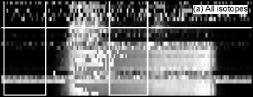
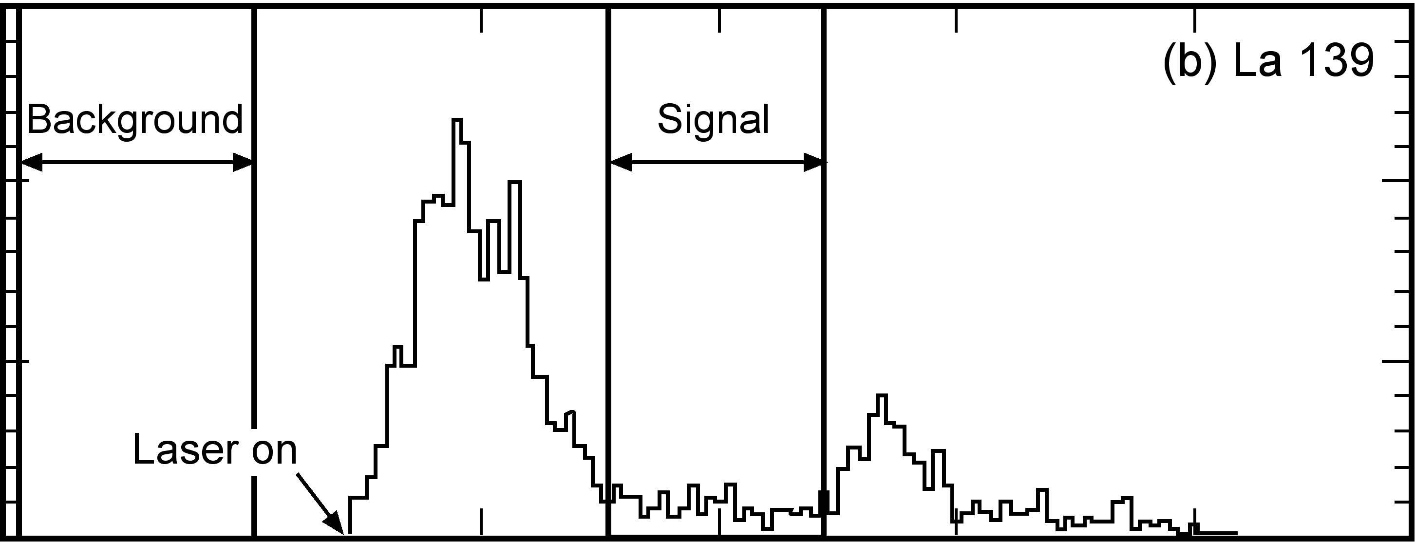
The "Review" window: Selection of background and signal intervals from the time-resolved signal is the key to rapid and accurate on-line analysis: this is done in GLITTER's unique "Review" window (Fig. 1). Two displays in "Review" show the time-resolved signals of the current analysis. The upper display consists of rows of pixels, each row representing the variation of the signal with time for a single isotope, with intensity shown by colour brightness (shades of grey in Fig.1). This gives an immediate and highly visible indication of any spikes in the data, or heterogeneity in the sample, for one or more isotopes. The lower display shows the time-resolved signal for a single isotope, selected using the horizontal marker in the upper display.

GLITTER initially calculates the results with default integration intervals, using a simple algorithm to avoid obvious heterogeneity and large spikes. Users can re-select the integration intervals for each analysis by simply dragging any of the four vertical markers in the "Review" window. As the markers are moved, the data are dynamically recalculated and updated in the results table and in any open "Plot" window(s). The use of GLITTER has led to a marked increase in the productivity of the LAM-ICPMS by allowing assessment of results before selection of the next point and eliminating off-line processing. More details are available at www.es.mq.au/GEMOC/.

Figure 1: GLITTER's "Review" window showing the time-resolved signals (X-axis = time, Y-axis = count rate) for an orthopyroxene grain where a rare earth element-rich inclusion was ablated near the start of the analysis. Note the high intensity area in the top half of (a), where the signals for the rare earth elements are shown. The integration interval was selected to avoid this part of the signal. The lower window (b) shows the signal for La 139.